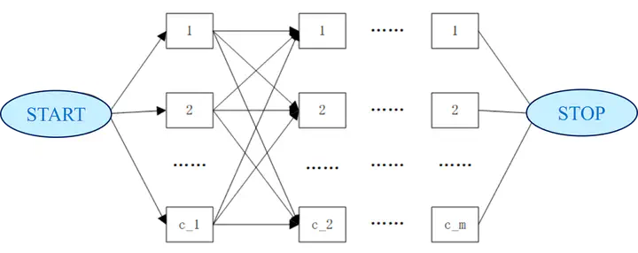
Lower Bounds for Hybrid Flow Shop Scheduling Problem

# We use the data from the reference[1]
job_data = [
    [3, 5, 9],
    [7, 1, 4],
    [2, 7, 4],
    [8, 2, 2],
    [6, 3, 7]
]

total_processing_times = [sum(jobs) for jobs in job_data]

makespan_lowerbound = max(total_processing_times)

import math

# we define a function of equation(4) in ref[1]
def stage_lb(list1, list2, list3, k):
    combined_sums = [x + y for x, y in zip(list2, list3)]

    min_value = min(combined_sums)
    combined_sums.remove(min_value)  # remove the minimum one
    second_min_value = min(combined_sums)  

    iso_sum = sum(list1)
    return 1/k*(iso_sum + min_value + second_min_value)

# Transfer the data
list1 = [item[0] for item in job_data]
list2 = [item[1] for item in job_data]
list3 = [item[2] for item in job_data]

k=2  # In each stage, we have 2 parallel processing machines.

# For each stage, we have：
stage_based_lowerbound1 = math.ceil(stage_lb(list1, list2, list3,k))
stage_based_lowerbound2 = math.ceil(stage_lb(list2, list1, list3,k))
stage_based_lowerbound3 = math.ceil(stage_lb(list3, list2, list1,k))

print("Stage 1 lower bound:", stage_based_lowerbound1)
print("Stage 2 lower bound:", stage_based_lowerbound2)
print("Stage 3 lower bound:", stage_based_lowerbound3)
print("Makespan lower bound:", makespan_lowerbound)